Predict Visitor Purchases with Google Analytics

20 Dec 2020

“The future depends on what we do in the present.” ― Mahatma Gandhi

Objective: The goal of this machine learning project is to develop a model that can predict whether or not a subset of visitors who returned to a website are likely to purchase.

For our task, we will use an ecommerce dataset that has millions of Google Analytics records for the Google Merchandise Store loaded into BigQuery. Using this data on each visitor session, we will build a model to get the probability of future purchase based on the data about their first session. Our binary classification model will be evaluated on ROC AUC, which is a number between 0 and 1, where 0 means 100% of the predictions are wrong and 1 means 100% of the predictions are correct. Randomly guessing should give a score of 0.5. With this model marketing teams could target those visitors with special promotions and ad campaigns.

Content (Notebook here):

Data Loading & Preparation
Data Exploration
Training and test dataset for batch prediction
Baseline & Model Evaluation
Model Training
Predictions
Model Analysis

The field definitions for the data-to-insights ecommerce dataset are here.

Important: For the purpose of our project, we will follow these steps in a linear fashion but machine learning pipeline is an iterative procedure.

Data Loading & Preparation

# BigQuery Query
from google.colab import auth
auth.authenticate_user()

project_id = '[YOUR PROJECT ID]'

data = pd.io.gbq.read_gbq(
'''
SELECT
    fullVisitorId,
    IFNULL(totals.bounces, 0) AS bounces,
    IFNULL(totals.timeOnSite, 0) AS time_on_site,
    IFNULL(totals.newVisits, 0) AS newVisits,
    IFNULL(totals.transactions, 0) AS transactions,
    IFNULL(totals.totalTransactionRevenue, 0) AS totalTransactionRevenue,
    date,
    visitStartTime,
    IFNULL(totals.pageviews, 0) AS pageviews,
    trafficSource.source,
    trafficSource.medium,
    channelGrouping,
    device.deviceCategory,
    geoNetwork.country
  FROM
    `data-to-insights.ecommerce.web_analytics` 

''', project_id=project_id, dialect='standard')

Processing & Description

# Copy
df = data.copy()

# Total transaction revenue were multiplied by 10^6
df['totalTransactionRevenue'] = df['totalTransactionRevenue']/1000000

# Adding Datetime features
df['date'] = pd.to_datetime(df['date'], format='%Y%m%d', errors='coerce')
df['visitStartTime_UTC'] = pd.to_datetime(df['visitStartTime'])
df["weekday"] = df['date'].dt.weekday
df["day"] = df['date'].dt.day
df["month"] = df['date'].dt.month
df["year"] = df['date'].dt.year
df['visitHour'] = (df['visitStartTime'].apply(lambda x: str(datetime.fromtimestamp(x).hour))).astype(int)
df['DayTime'] = pd.cut(df['visitHour'],[0,6,12,18,24],labels=['Night','Morning','Afternoon','Evening']).astype(object)
df['DayTime'] = df['DayTime'].fillna('Other')
print(df.shape)

# Exploratory Data Analysis
EDA = pd.DataFrame(columns = ['Columns','Types','Values', 'Uniques', 'Uniques(no nulls)', 'Missing(n)', 'Missing(%)'])
eda = pd.DataFrame()

for c in df.columns:
    eda['Columns'] = [c]
    eda['Types'] = df[c].dtypes
    eda['Values'] = [df[c].unique()]
    eda['Uniques'] = len(list(df[c].unique()))
    eda['Uniques(no nulls)'] = int(df[c].nunique())
    eda['Missing(n)'] = df[c].isnull().sum()
    eda['Missing(%)'] = (df[c].isnull().sum()/ len(df)).round(3)*100
    EDA = EDA.append(eda)
EDA

Target column

Note that when working with binary classification problems, especially imbalanced problems, it is important that the majority class is assigned to class 0 and the minority class is assigned to class 1. This is because many evaluation metrics will assume this relationship.

df['NextPurchase'] = 0
df.loc[(df['transactions'] > 0) & (df['newVisits'] == 0 ) ,'NextPurchase'] = 1

# summarize the class distribution
target = df['NextPurchase'].values
counter = Counter(target)
for k,v in counter.items():
  per = v / len(target) * 100
  print('Class=%d, Count=%d, Percentage=%.1f%%' % (k, v, per))

Class=0, Count=955782, Percentage=98.5%

Class=1, Count=14750, Percentage=1.5%

Data Exploration

What % of the total visitors made a purchase?

purcharsers = df.loc[df['transactions'] > 0]
purchasers = purcharsers.groupby('fullVisitorId').transactions.sum().reset_index()
result = purchasers.fullVisitorId.nunique()/ df.fullVisitorId.nunique()*100
print('{:.1f}% of the total visitors made a purchase'.format(result))

2.7% of the total visitors made a purchase

What % of visitors bought on subsequent visits to the website?

result = df.groupby('NextPurchase').fullVisitorId.nunique()[1]/df.groupby('NextPurchase').fullVisitorId.nunique()[0]*100
print('{:.1f}% of the total visitors will return and purchase from website'.format(result))

1.6% of the total visitors will return and purchase from website

Training & test dataset for batch prediction

Training on 11 months of session data
1 month for test

train = df[df.date.between('20160801', '20170630')] # 11 months
test = df[df.date.between('20170701', '20170801')] # 1 month

# Train & Validation
X, y = train[['bounces', 'time_on_site','pageviews',
              'source', 'channelGrouping', 'deviceCategory',
              'country','DayTime']], train.NextPurchase

Baseline & Model Evaluation

Baseline

Our dataset has a 98.5%/1.5% class distribution for the majority and minority classes. This distribution can be predicted for each example to give a baseline for probability predictions.

# Baseline Logloss
distribution = train['NextPurchase'].value_counts()
majority = distribution[0]
minority = distribution[1]
probabilities = [[majority, minority] for _ in range(len(y))]
avg_logloss = log_loss(y, probabilities)

# Baseline ROC AUC
model = DummyClassifier(strategy='stratified')
cval = RepeatedStratifiedKFold(n_splits=10, n_repeats=1, random_state=1)
scores = cross_val_score(model, X, y, scoring='roc_auc', cv=cval, n_jobs=-1)

print('Baseline: Log Loss: %.3f' % (avg_logloss))
print('Baseline: ROC AUC: %.3f (%.3f)' % (mean(scores), std(scores)))

Baseline: Log Loss: 0.693

Baseline: ROC AUC: 0.500 (0.002)

As expected, the no-skill classifier achieves a mean ROC AUC of 0.5. This provides a baseline in performance, above which a model can be considered skillful on this dataset. Alternatively, a Logloss scores below 0.69 will also represent a model that has some skill.

Cross-Validation for Imbalanced Classification

We will use mostly default model hyperparameters, with the exception of the class weight parameter, which we will set to ‘Balance’ in order to make our algorithm cost-sensitive for our task.

CatBoost is an open-sourced gradient boosting library. One of the differences between CatBoost and other gradient boosting libraries is its advanced processing of the categorical features. We can use CatBoost without any explicit pre-processing to convert categories into numbers. CatBoost converts categorical values into numbers using various statistics on combinations of categorical features and combinations of categorical and numerical features.

cat_features = np.where(X.dtypes == object)[0] # categorical variables

model = CatBoostClassifier()
cv_params = model.get_params()

# Stratified is turned on (True) by default if Logloss is selected 
cv_params = {'eval_metric': 'Logloss',
             'custom_metric': ['AUC','Precision', 'Recall'],
             'random_seed': 42, 
             'iterations': 150, 
             'loss_function' : 'Logloss',
             'auto_class_weights' :'Balanced',
             'early_stopping_rounds' : 10}

cv_data = cv(Pool(X, y, cat_features=cat_features), cv_params, seed=17, fold_count=5, verbose=True)

print('Best validation Logloss: {:.2f}±{:.4f} on step {}'.format(np.min(cv_data['test-Logloss-mean']),
    cv_data['test-Logloss-std'][np.argmin(cv_data['test-Logloss-mean'])],
    np.argmin(cv_data['test-Logloss-mean'])))
print('Best validation ROC AUC score: {:.2f}±{:.4f} on step {}'.format(np.max(cv_data['test-AUC-mean']),
    cv_data['test-AUC-std'][np.argmax(cv_data['test-AUC-mean'])],
    np.argmax(cv_data['test-AUC-mean'])))

The results suggest that the CatBoost algorithm performs well, achieving a mean ROC AUC above the naive model with 0.98.

Model Training

%%time
cat_features = np.where(X.dtypes == object)[0]
model = CatBoostClassifier(iterations=150, random_seed=42, loss_function = 'Logloss', auto_class_weights='Balanced')
model.fit(X, y, cat_features=cat_features, verbose=False)

Predictions

We will use our model to predict the probability that a first-time visitor to the Google Merchandise Store will make a purchase in a later visit. To do that, we will use our test dataset and predict which new visitors will come back and purchase.

np.set_printoptions(precision=2)

X_test, y_test = test[['bounces', 'time_on_site','pageviews',
       'source', 'channelGrouping', 'deviceCategory', 'country','DayTime']], test.NextPurchase


titles_options = [("Confusion matrix, without normalization", None),
                  ("Normalized confusion matrix", 'true')]
for title, normalize in titles_options:
    disp = plot_confusion_matrix(model, X_test, y_test,
                                 display_labels=['Not purchase', 'Purchase'],
                                 cmap=plt.cm.Blues,
                                 normalize=normalize)
    disp.ax_.set_title(title)

    print(title)
    print(disp.confusion_matrix)

plt.show()

# ROC AUC
curve = get_roc_curve(model, Pool(X_test, y_test, cat_features=cat_features))
(fpr, tpr, thresholds) = curve
roc_auc = auc(fpr, tpr)
print()
print('ROC AUC: %.3f' % (roc_auc))

ROC AUC: 0.978

The reported performance is good, but not highly optimized (e.g. hyperparameters are not tuned).

Model Analysis (Interpretability)

In this section, we will try to understand how the model makes predictions.

Which features had the biggest impact ?

shap.initjs()
explainer = shap.TreeExplainer(model)
shap_values = explainer.shap_values(X_test)
shap.summary_plot(shap_values, X_test, plot_type="bar")

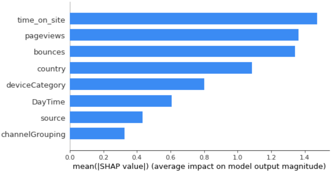
We can see that time_on_site, pageviews and bounces are the top 3 feautures.

Now, let’s use a summary plot of the SHAP values.

shap.initjs()
explainer = shap.TreeExplainer(model)
shap_values = explainer.shap_values(X_test)
shap.summary_plot(shap_values, X_test)

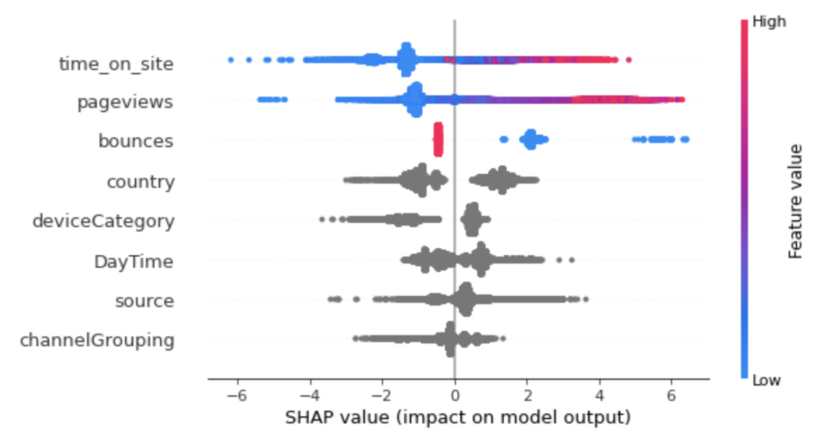
High values of time_on_site and pageviews caused higher predictions, and low values caused low predictions.
Low values of bounces caused higher predictions, and high values caused low predictions.
The country, device and channelGrouping affect the prediction.

Louis Willems