Applying Data Science to E-commerce
10 Mar 2020“Documentation is a love letter that you write to your future self.” ― Damian Conway
In this post, I will try to apply Data Science methods to an eCommerce business. To do so, we will extract the dataset of an online retail from Kaggle then we will analyse the data. Here, I did my best to follow a comprehensive, but not exhaustive, analysis of E-commerce data. I’m far from reporting a rigorous analysis in this post, but I hope that it can be useful.
Content (Notebook here):
- E-commerce Data Analysis
- Customer Segmentation
- Predicting Next Purchase Day
- Forecasting Revenue
1. E-commerce Data Analysis
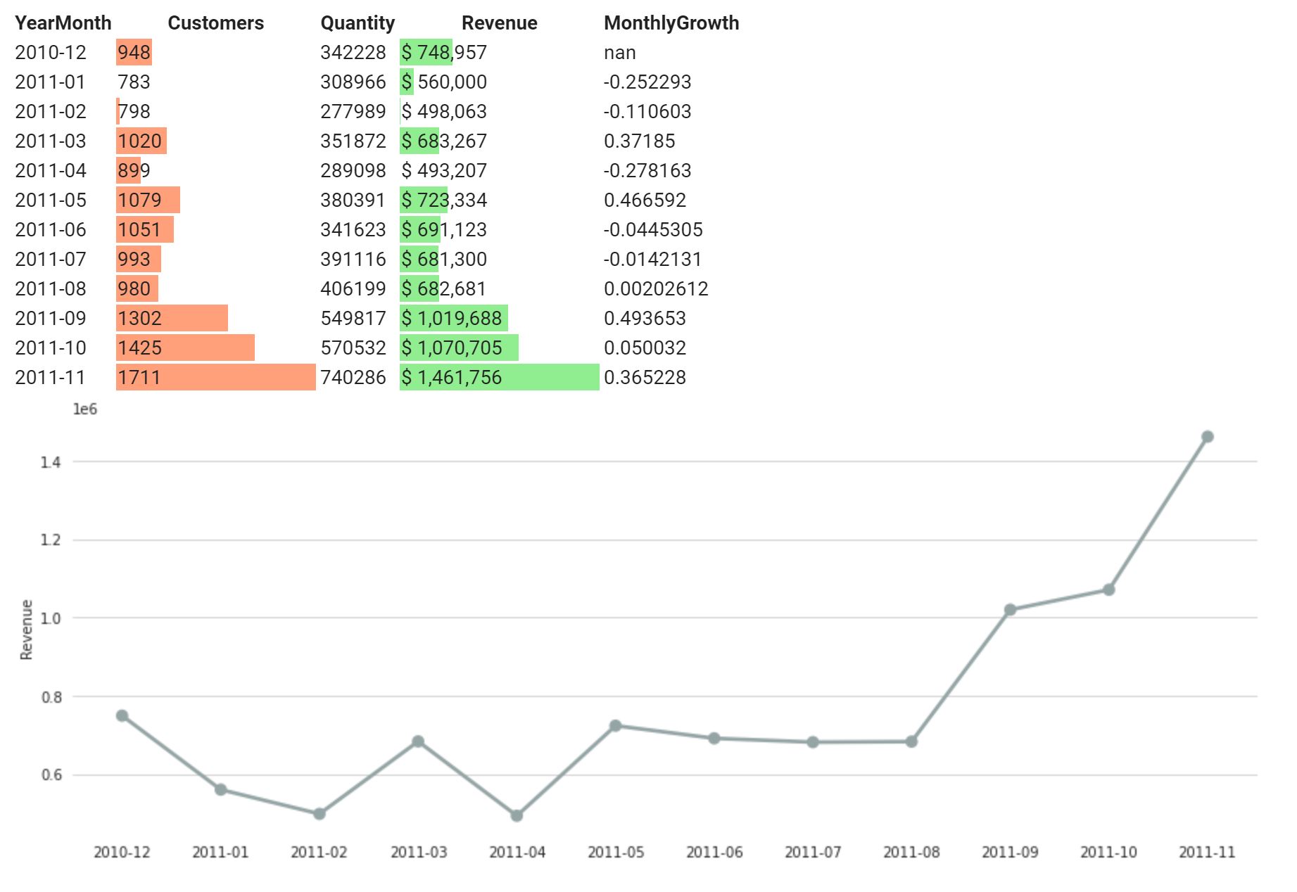
Revenue & Growth Rate
# Monthly data
df_monthly = df.copy()
df_monthly = df_monthly.groupby('YearMonth').agg({'CustomerID': lambda x: x.nunique(), 'Quantity': 'sum', 'Revenue': 'sum', }).reset_index()
df_monthly['YearMonth'] = df_monthly['YearMonth'].astype(str)
df_monthly['YearMonth']= df_monthly['YearMonth'].str.split('(\d{4})(\d{2})').str.join('-').str.strip('-')
df_monthly['YearMonth'] = df_monthly['YearMonth'].astype('category')

# Monthly Growth %
df_monthly['MonthlyGrowth'] = df_monthly['Revenue'].pct_change()
# df_monthly['MonthlyGrowth'] = df_monthly['MonthlyGrowth'].apply("{:,.1f}%".format)
df_monthly.columns = ['YearMonth', 'Customers', 'Quantity', 'Revenue', 'MonthlyGrowth']
df_monthly['Customers'] = df_monthly['Customers'].astype(int)


sns.set_style("whitegrid")
sns.catplot(x="YearMonth", y="Revenue", data=df_monthly, kind="point", aspect=2.5, color="#95a5a6")
plt.ylabel('Revenue')
plt.xlabel('')
sns.despine(left=True, bottom=True)

df_monthly.style.format({"Customers": "{:.0f}",
                             "Quantity": "{:.0f}",
                             "Revenue": "${:20,.0f}"})\
                    .hide_index()\
                    .bar(subset=["Revenue",], color='lightgreen')\
                    .bar(subset=["Customers"], color='#FFA07A')
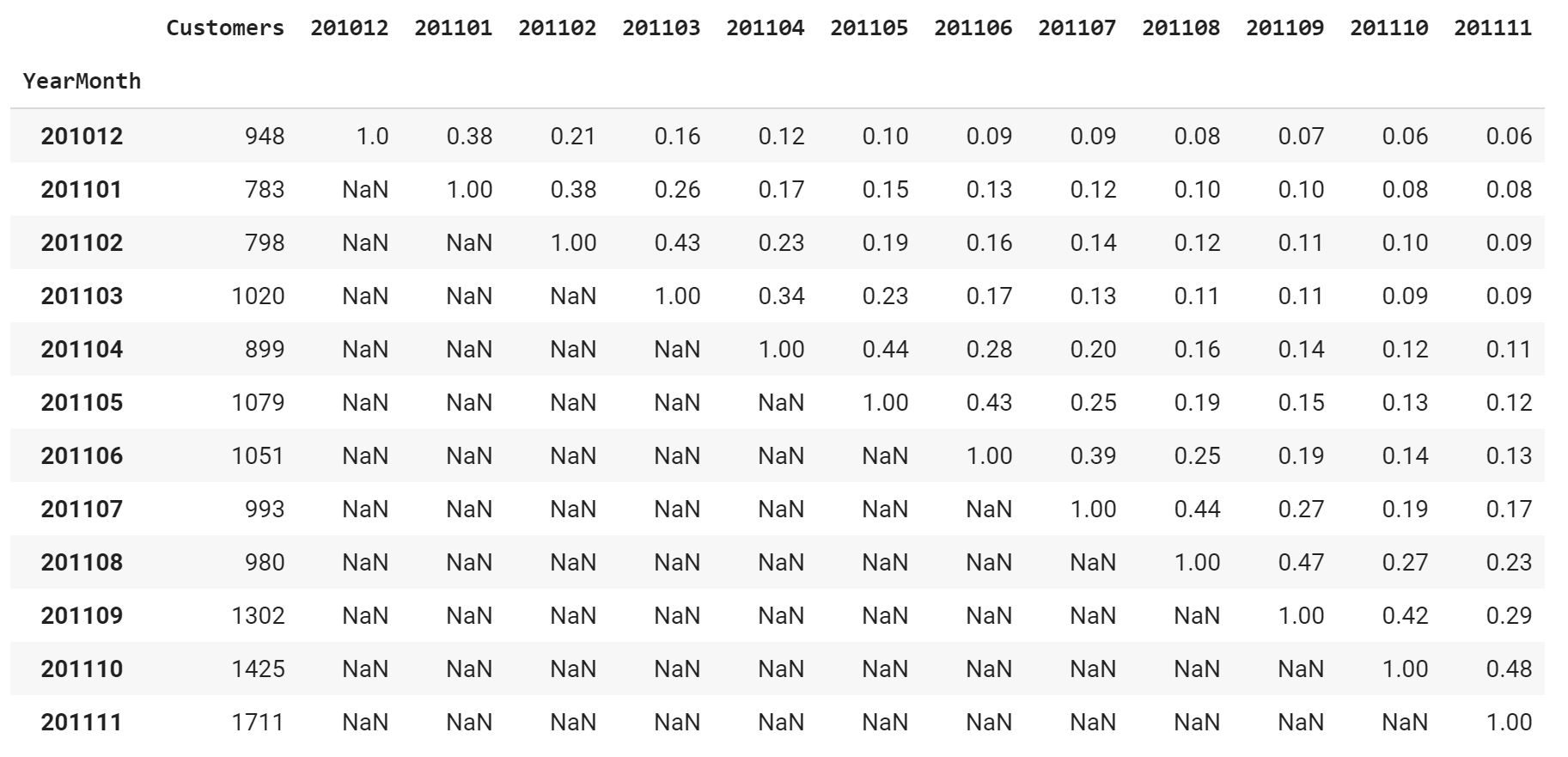
Cohort Based Analysis
A cohort analysis is the process of analyzing the behavior of groups of users who share a common characteristic. Here, the common characteristic is identified by the first purchase in each month.
df_cohort = pd.crosstab(df_customer_monthly_revenue['CustomerID'], df_customer_monthly_revenue['YearMonth']).reset_index()

new_column_names = [ 'm_' + str(column) for column in df_cohort.columns]
df_cohort.columns = new_column_names

#Retained customers for each cohort monthly
retention_array = []
for i in range(len(months)):
    retention_data = {}
    selected_month = months[i]
    prev_months = months[:i]
    next_months = months[i+1:]
    for prev_month in prev_months:
        retention_data[prev_month] = np.nan

    total_user_count =  retention_data['Customers'] = df_cohort['m_' + str(selected_month)].sum()
    retention_data[selected_month] = 1

    query = "{} > 0".format('m_' + str(selected_month))

    for next_month in next_months:
        query = query + " and {} > 0".format(str('m_' + str(next_month)))
        retention_data[next_month] = np.round(df_cohort.query(query)['m_' + str(next_month)].sum()/total_user_count,2)
    retention_array.append(retention_data)

df_cohort = pd.DataFrame(retention_array)
df_cohort.index = months
df_cohort
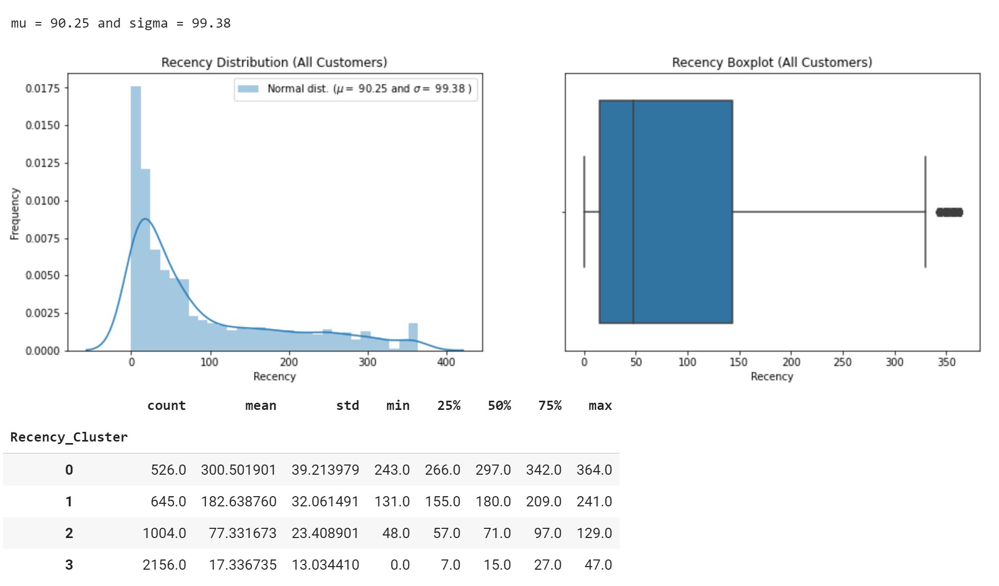
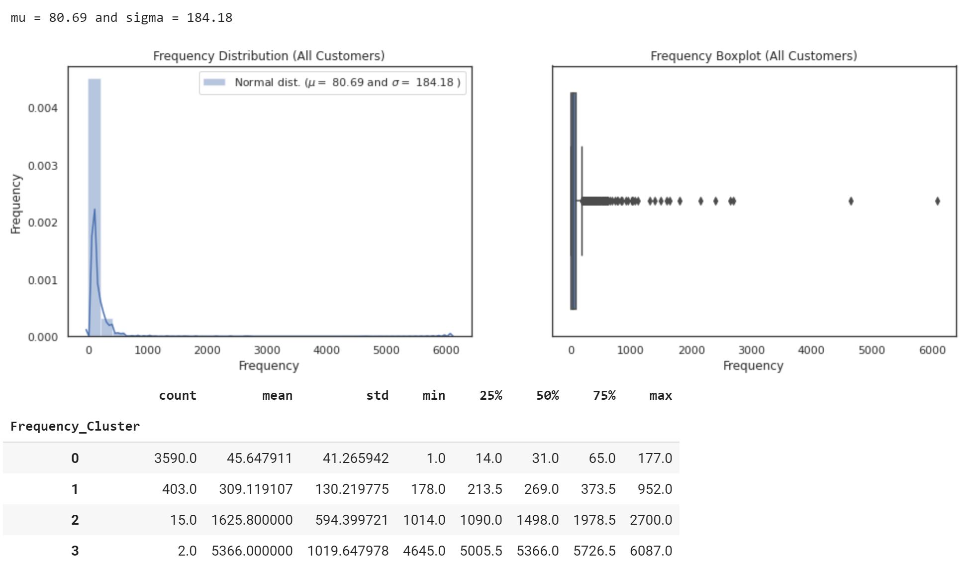
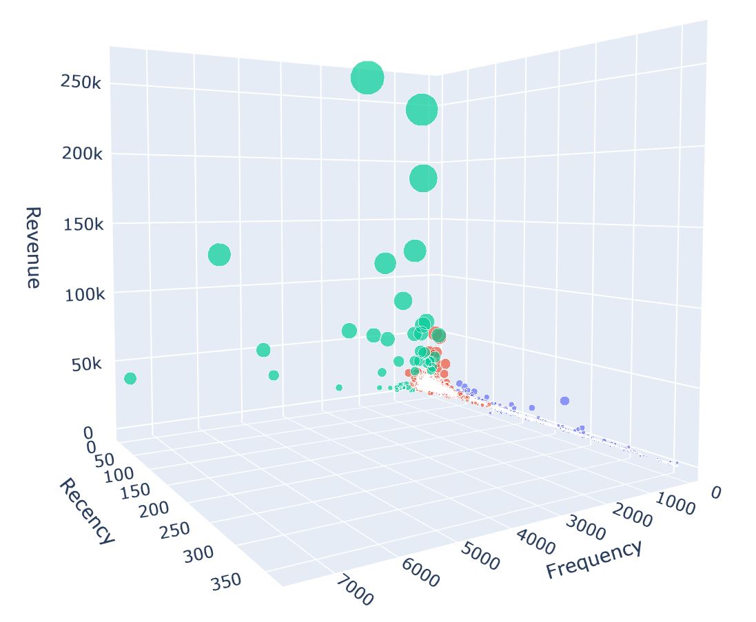
2. Customer Segmentation (RFM Clustering)
In order to create our customer segments, we will use the RFM method. We will calculate Recency, Frequency and Monetary and apply unsupervised machine learning to identify our different segments:
- Not Engaged
- Engaged
- Best
For RFM clustering, instead of using kmeans, we will use Fisher-Jenks algorithm (Jenks optimization or natural breaks) that is a little more intuitive. For the purposes of this article, I will use jenkspy from Matthieu Viry.
Recency (Inactive days)
Frequency (Number of orders)
Monetary (Revenue)

3. Predicting Next Purchase
In this section, we will try to predict if a customer is likely to make a new purchase. For this, we will use 9 months of data to predict if a customer will make another order in the next 40 days.
# Next Purchase data
df_9m = df[df.date.between('12-01-2010', '08-31-2011')]
df_3m = df[df.date.between('09-01-2011', '11-30-2011')]

pred_user = pd.DataFrame(df_9m['CustomerID'].unique())
pred_user.columns = ['CustomerID']

next_3m = df_3m.groupby('CustomerID').InvoiceDate.min().reset_index()
next_3m.columns = ['CustomerID','MinPurchaseDate']

last_9m = df_9m.groupby('CustomerID').InvoiceDate.max().reset_index()
last_9m.columns = ['CustomerID','MaxPurchaseDate']

user_m = pd.merge(last_9m, next_3m,on='CustomerID',how='left')
user_m['NextPurchaseDay'] = (user_m['MinPurchaseDate'] - user_m['MaxPurchaseDate']).dt.days

user_next = pd.merge(pred_user, user_m[['CustomerID','NextPurchaseDay']],on='CustomerID',how='left')
user_next = user_next.fillna(0)
print(user_next.shape)
Feature Engineering
For our classification problem, we will create the features below:
- RFM scores & clusters
- Days between the last three purchases
- Mean & standard deviation of the difference between purchases in days
Target
For our binary classification, the target variable will be creted as follow:
- Class 0 — Customers that will purchase in 0–40 days
- Class 1 — Customers that will purchase in more than 2 months (≥ 40)
df_next = predict.copy()
df_next['NextPurchaseDayRange'] = 0
df_next.loc[df_next.NextPurchaseDay>40,'NextPurchaseDayRange'] = 1
df_next['NextPurchaseDayRange'].value_counts(normalize=True)*100
Binary Classification
#Train & Validation
dataset = df_next.drop(['NextPurchaseDay', 'CustomerID', 'Frequency_Cluster','DayDiff'],axis=1)
X, y = dataset.drop('NextPurchaseDayRange',axis=1), dataset.NextPurchaseDayRange

X_train, X_valid, y_train, y_valid = train_test_split(X, y, test_size=0.2, random_state=44)

model = CatBoostClassifier(iterations=150,random_seed=42,eval_metric='AUC',logging_level='Silent')
model.fit(X_train, y_train, eval_set=(X_valid, y_valid))

cv_params = model.get_params()
print('cv params: ', cv_params)

cv_data = cv(
    Pool(X, y),
    cv_params,
    seed=17,
    fold_count=5
)

print('Best validation accuracy score: {:.2f}±{:.4f} on step {}'.format(np.max(cv_data['test-AUC-mean']),
    cv_data['test-AUC-std'][np.argmax(cv_data['test-AUC-mean'])],
    np.argmax(cv_data['test-AUC-mean'])
))
cv params: {‘eval_metric’: ‘AUC’, ‘logging_level’: ‘Silent’, ‘random_seed’: 42, ‘iterations’: 150} Best validation accuracy score: 0.77±0.0366 on step 64
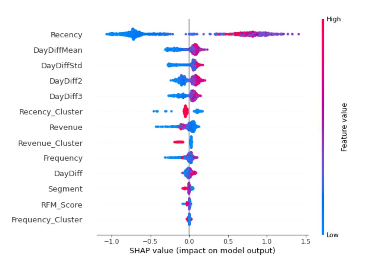
Model Analysis (Interpretability)
In this section, we will try to understand how the model makes predictions.
What features in the data did the model think are most important?
import shap
shap.initjs()

explainer = shap.TreeExplainer(model)
shap_values = explainer.shap_values(X)

#  effects of all the features
shap.summary_plot(shap_values, X)
4. Forecasting Revenue
Forecasting daily or monthly revenue can be used for planning budgtes/targets or as a benchmark.
Choice of forecasting methods is on a case by case basis depending on the nature of the dataset. Some of these methods include Moving Average, Exponential Smoothing (Simple, Double), Holt-Winters, ARIMA, SARIMA, LSTM and Prophet among others.
In this section, we will forecast with Prophet (15 days). Prophet is very powerful and effective in time series forecasting. It works best with time series that have strong seasonal effects and several seasons of historical data.
# MAPE
def mean_absolute_percentage_error(y_true, y_pred):
    y_true, y_pred = np.array(y_true), np.array(y_pred)
    return np.mean(np.abs((y_true - y_pred) / y_true)) * 100

# Copy
df_forecast = df.copy()
df_forecast = df_forecast.groupby('date').Revenue.sum().reset_index()


# Train & Valid
periods=15
df_forecast.columns = ['ds','y']
train_data = df_forecast.iloc[:len(df_forecast)- periods]
valid_data = df_forecast.iloc[len(df_forecast)-periods:]


# Model Optimization
m = Prophet(seasonality_mode='multiplicative', changepoint_prior_scale=0.5, seasonality_prior_scale= 10)
m.add_seasonality(name='daily', period=1, fourier_order=15)
m.add_seasonality(name='weekly', period=7, fourier_order=20)
m.add_seasonality(name='monthly', period=30.5, fourier_order=12)
m.add_country_holidays(country_name='CA')
m.fit(train_data)
future = m.make_future_dataframe(periods=periods)

forecast = m.predict(future)

# Predictions
prophet_pred = pd.DataFrame({"Date" : forecast[-periods:]['ds'], "Pred" : forecast[-periods:]["yhat"]})
prophet_pred = prophet_pred.set_index("Date")
valid_data["Prophet_Predictions"] = prophet_pred['Pred'].values
print('Baseline MAPE: {}'.format(mean_absolute_percentage_error(valid_data["y"], valid_data["Prophet_Predictions"])))

# Visualization
plt.figure(figsize=(16,5))
ax = sns.lineplot(x= df_forecast.ds, y=df_forecast["y"])
sns.lineplot(x=valid_data.ds, y = valid_data["Prophet_Predictions"]);
plt.title("Forecasted Value vs Actuals")
plt.show()
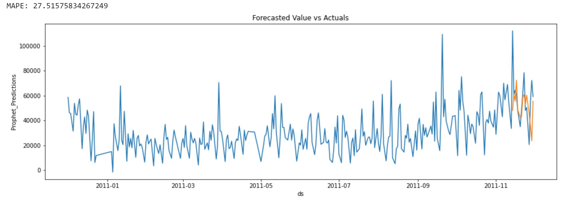
We get a MAPE of 27.5%. Not a really a good predcition. This indicates that over all the points predicted, we are out with an average of 27.5% from the true value.
Typical forecasting errors are around 5% for predictions of one month and 11% for one year.